Deep Learning with GPU- How do we start? — A quick setup guide on Amazon ec2

Deep learning is one of the hottest buzzwords in tech and is impacting everything from health care to transportation to manufacturing, and more. Companies are turning to deep learning to solve hard problems, like speech recognition, object recognition, and machine translation.

Everything new breakthrough comes with challenges. The biggest challenge for deep learning is that it requires intensive training of the model and massive amount of matrix multiplications and other operations. A single CPU usually has no more than 12 cores and it will be a bottleneck for deep learning network development. The good thing is that all the matrix computation can be parallelized and that’s where GPU comes into rescue. A single GPU might have thousands of cores and it is a perfect solution to deep learning’s massive matrix operations. GPUs are much faster than CPUs for deep learning because they have orders of magnitude more resources dedicated to floating point operations, running specialized algorithms ensuring that their deep pipelines are always filled.

The good thing is that all the matrix computation can be parallelized and that’s where GPU comes into rescue. A single GPU might have thousands of cores and it is a perfect solution to deep learning’s massive matrix operations. GPUs are much faster than CPUs for deep learning because they have orders of magnitude more resources dedicated to floating point operations, running specialized algorithms ensuring that their deep pipelines are always filled.

GPUs are much faster than CPUs for deep learning because they have orders of magnitude more resources dedicated to floating point operations, running specialized algorithms ensuring that their deep pipelines are always filled.

Now we’re know why GPU is necessary for deep learning. Probably you’re interested in deep learning and can’t wait to do something about it. But you don’t have big GPUs on your computer. The good news is that there are public GPU serves for you to start with. Google, Amazon, OVH all have GPU servers for you to rent and the cost is very reasonable.

In this article, I’ll show you how to set up a deep learning server on Amazon ec2, p2-2xlarge GPU instance in this case. In order to set up amazon instance, here is the prerequisite software you’ll need:

1. Python 2.7 (recommend anaconda)
2. Cygwin with wget, vim (if on windows)
3. Install Amazon AWS Command Line Interface (AWS CLI), for Mac

Here is the fun part:

1. Register an Amazon ec2 account at: https://aws.amazon.com/console/
2. Go to Support –> Support Center –> Create case  (Only for the new ec2 user.)Type in the information in the form and ‘submit’ at the end. Wait for up to 24-48 hours for it to be activated. If you are already an ec2 user, you can skip this step.
3. Create new user group. From console, Services –> Security, Identity & Compliance –> IAM –> Users –> Add user
4. After created new user, add permission to the user by click the user just created.
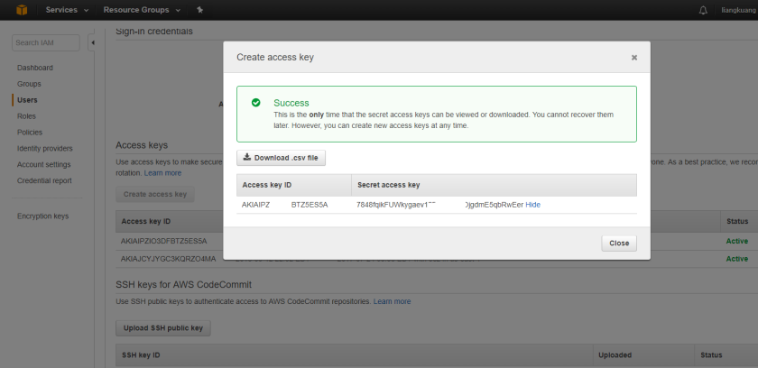
5. Obtain Access keys: Users –> Access Keys –> Create access key. Save the information.
6. Now we’re done with Amazon EC2 account, go to Mac Terminal or Cygwin on Windows
7. Download set-up files from fast.ai. setup_p2.sh and setup_instance.sh . Change the extension to .sh since WordPress doesn’t support bash file upload
8. Save the two shell script to your current working directory
9. In the terminal, type: aws configure                                                                                      Type in the access key ID and Secret access key saved in step 5.
10. bash setup_p2.sh
11. Save the generated text (on terminal) for connecting to the server
12. Connect to your instance: ssh -i /Users/lxxxx/.ssh/aws-key-fast-ai.pem ubuntu@ec2-34-231-172-2xx.compute-1.amazonaws.com
13. Check your instance by typing: nvidia-smi
14. Open Chrome Browser with URL: ec2-34-231-172-2xx.compute-1.amazonaws.com:8888Password: dl_course
15. Now you can start to write your deep learning code in the Python Notebook.
16. Shut down your instance in the console or you’ll pay a lot of money.

For a complete tutorial video, please check Jeremy Howard’s video here.

Tips:

The settings, passwords are all saved at ~/username/.aws , ~/username/.ipython.

 

 

 

 

The convenience of subplot = True in dataframe.plot

When it comes to data analysis, there is always a saying: “one picture worths a thousand words.”. Visualization is an essential and effective way of data exploration and usually as our first step of understanding the raw data. In Python, there are a lot of visualization libraries. For python dataframe, it has plenty of built-in plotting methods: line, bar, barh, hist, box, kde, density, area, pie, scatter and hexbin.

The quickest way to visualize all the columns data in a dataframe can be achieved by simply call: df.plot().  For example:

df = pd.DataFrame({‘A’:np.arange(1,10),’B’:2*np.arange(1,10)})
df.plot(title = ‘plot all columns in one chart.’)

But a lot of times we want each feature plotted on a separate chart due to the complex of data. It will help us disentangle the dataset.

It turns out that there is a simple trick to play with in df.plot, using ‘subplot = True’.

df.plot(figsize = (8,4), subplots=True, layout = (2,1), title = ‘plot all columns in seperate chart’);

That’s it. Simple but effective. You can change the layout by playing with the layout tupple input.

Hope you find it helpful too.

All about *apply family in R

R has many *apply functions which are very helpful to simplify our code. The *apply functions are all covered in dplyr package but it is still good to know the differences and how to use it. It is just too convenient to ignore them.

First, the following Mnemonics gives you an overview of what each *apply function do in general.

Mnemonics

• lapply is a list apply which acts on a list or vector and returns a list.
• sapply is a simple lapply (function defaults to returning a vector or matrix when possible)
• vapply is a verified apply (allows the return object type to be prespecified)
• rapply is a recursive apply for nested lists, i.e. lists within lists
• tapply is a tagged apply where the tags identify the subsets
• apply is generic: applies a function to a matrix’s rows or columns (or, more generally, to dimensions of an array)

Example:

apply
For sum/mean of each row/columns, there are more optimzed function: colMeans, rowMeans, colSums, rowSums.While using apply to dataframe, it will automatically coerce it to a matrix.

# Two dimensional matrix# Two dimensional matrix
myMetric <- matrix(floor(runif(15,0,100)),5,3)
myMetric
# apply min to rows
apply(myMetric,1,min)
# apply min to columns
apply(myMetric,2,min)

[,1] [,2] [,3]
[1,] 28 22 6
[2,] 31 75 80
[3,] 7 88 96
[4,] 15 70 27
[5,] 74 84 12 //
[1] 6 31 7 15 12 //
[1] 7 22 6 //

lapply
For list vector, it applies the function to each element in it. lapply is the workhorse under all * apply functions. The most fundamental one.

x <- list(a = runif(5,0,1), b = seq(1:10), c = seq(10:100))
lapply(x, FUN = mean)

# Result

$a
[1] 0.4850281

$b
[1] 5.5

$c
[1] 46

sapply
sapply is doing the similar to lapply, it is just the output different. It simplifies the output to a vector rather than a list.

x <- list(a = runif(5,0,1), b = seq(1:10), c = seq(10:100))
sapply(x, FUN = mean)

a                 b                  c
0.2520706 5.5000000 46.0000000

vapply – similar to sapply, just speed faster.

rapply
This is a recursive apply, especially useful for a nested list structure. For example:

#Append ! to string, otherwise increment
myFun <- function(x){
if (is.character(x)){
return(paste(x,”!”,sep=””))
}
else{
return(x + 1)
}
}

#A nested list structure
l <- list(a = list(a1 = “Boo”, b1 = 2, c1 = “Eeek”),
b = 3, c = “Yikes”,
d = list(a2 = 1, b2 = list(a3 = “Hey”, b3 = 5)))

#Result is named vector, coerced to character
rapply(l,myFun)

#Result is a nested list like l, with values altered
rapply(l, myFun, how = “replace”)

a.a1 a.b1 a.c1 b c d.a2 d.b2.a3 d.b2.b3
“Boo!” “3” “Eeek!” “4” “Yikes!” “2” “Hey!” “6”

[1] “break”
$a
$a$a1
[1] “Boo!”

$a$b1
[1] 3

$a$c1
[1] “Eeek!”

 

$b
[1] 4

$c
[1] “Yikes!”

$d
$d$a2
[1] 2

$d$b2
$d$b2$a3
[1] “Hey!”

$d$b2$b3
[1] 6

tapply
For when you want to apply a function to subsets of a vector and the subsets are defined by some other vector, usually a factor.

tapply is similar in spirit to the split-apply-combine functions that are common in R (aggregate, by, avg, ddply, etc.)

x <- 1:20
y = factor(rep(letters[1:5], each = 4))
tapply(x,y,sum)

a b c d e
10 26 42 58 74

mapply and map
For when you have several data structures (e.g. vectors, lists) and you want to apply a function to the 1st elements of each, and then the 2nd elements of each, etc., coercing the result to a vector/array as in sapply.

**Map** is a wrapper to mapply with SIMPLIFY = FALSE, so it will be guaranteed to return a list.

mapply(sum, 1:5, 1:10,1:20)
mapply(rep, 1:4, 4:1)

[1] 3 6 9 12 15 13 16 19 22 25 13 16 19 22 25 23 26 29 32 35
[[1]]
[1] 1 1 1 1

[[2]]
[1] 2 2 2

[[3]]
[1] 3 3

[[4]]
[1] 4

 

This post is compiled from stackoverflow’s top answers.

A better view of this is to look at the R Notebook I’ve created: https://rpubs.com/euler-tech/292794

Access Amazon Redshift Database from Python

Amazon has definitely made significant gain from the cloud movement in the past decade as more and more company are ditching their own data server in favor of theirs. There is a very good reason to do that. Cheaper, faster and easy access from anywhere.

Now how do we retrieve data in Redshift and do data analysis from Python. It is very simple to do that. The information that you’ll need ahead is: usename, password, url to redshift and port number (default is 5439).

I’ll show you how to connect to Amazon Redshift using psycopg2 library. First install library ‘psycopg2’ using : pip install psycopg2.

Then use the following Python code to define your connections.

def create_conn(*args, **kwargs):

import psycopg2
config = kwargs['config']
try:
con = psycopg2.connect(dbname = config['dbname'], host=config['host'],
port = config['port'], user=config['user'],
password=config['pwd'])
return con
except Exception as err:
print(err)

keyword= getpass('password')   # type in password  or you can read from a saved json file.

config = {'dbname': 'lake_one',
'user':'username',
'pwd':'keyword',
'host':'[your host url].redshift.amazonaws.com',
'port':5439}

How to use this and do fun stuff:

con = create_conn(config = config)
data = read_sql("select *  from mydatabase.tablename;",con, index_col = 'date')
print(data.columns)
data.plot(title='My data', grid = True,figsize=(15,5))

con.close() # close connection

Simple as that. Now it’s your turn to create fantastic analysis.

How to use customized function for any Pipe operator %>% in R

For advanced R programmer or Python (spark) machine learning engineer, you probably have heard or used at least once pipeline for your data or model work flow. The concept of pipeline is derived from Unix/Linux shell command. A pipeline is a sequence of processes chained together by their standard streams so that the output of each process (stdout) feeds directly as input (stdin) to the next one, for example: ls -l | grep key
less. Since the debut of one of the greatest R package ‘magrittr‘, pipeline has been one of my favorite thing in data engineering.

As we know, the way pipeline requires you to pass the whole output from previous command [process] to next one. Here comes a problem when you want use some basic/simple R command for just a particular column in the data object. For example, if I have a dataset ‘babynames’ and I want to round the ‘prop’ column to 3 digits. What will happen if I do this:

library(babynames)
library(dplyr)
library(magrittr)

babynames %>%
round(‘prop’) %>%
head

It gives me an error:

babynames %>%
+ round(‘prop’) %>%
+ head
Error in Math.data.frame(list(year = c(1880, 1880, 1880, 1880, 1880, 1880, :
non-numeric variable in data frame: sexname

How am I going to fix it? The solution is simple, write a customized wrapper function to let it go with the flow. Here is the solution:

library(babynames)
library(dplyr)
library(magrittr)

myRound <- function(df,colname){
df[[colname]] <- round(df[[colname]], 3)
return(df)
}

babynames %>%
myRound(‘prop’) %>%
head

Now it works. Whooray!

year sex name n prop
<dbl> <chr> <chr> <int> <dbl>
1 1880 F Mary 7065 0.072
2 1880 F Anna 2604 0.027
3 1880 F Emma 2003 0.021
4 1880 F Elizabeth 1939 0.020
5 1880 F Minnie 1746 0.018
6 1880 F Margaret 1578 0.016

Why it works?

The way pipeline works are like going through a multiple-stage filter for a signal, it can only take the whole object as input instead part of it. So the wrapper function operates as a buffer function within the pipeline.

 

Can’t start Jupyter Notebook in macOS Sierra 10.12.5

Many people have experienced an annoying issue after updating to macOS Sierra 10.12.5 while trying to fire up the Jupiter notebook. There are two sequential ways of fixing the issue depends on your Mac environment.

The first easy fix is to copy and paste: http://localhost:8888/tree directly into your browser. If doesn’t work in Chrome, using Safari.

What I found out the more annoying issue is that the first fix simply won’t do it, and it prompts you to enter a password after pasting the link into browser. This problem can be fixed by changing the Jupiter notebook server settings. Simply by following the steps:

1. Open Mac Terminal

2. jupyter notebook –generate-config 

   This command generate config file under

   /Users/[username]/.jupyter/

3. jupyter notebook password

Type in your password twice and it will save the hashed password into      ./jupyter/jupyter_notebook_config.json

After this setting, fire up your notebook and type in your previous password (not hashed value) and save it. It will not ask for password anymore.

Some helpful command to use:

jupyter –version

jupyter notebook list  : list all running notebook sesion

If you still have problem, combine two steps together and it should work.

 

 

Converting week numbers to dates

While working with time series dataset, sometimes you’ll only get the date as week number of its residing year. This articles presents easy way to convert it to datetime tuple and datetime object in Python.

Easy way to do it is using strptime from the datetime module. Example:

import datetime

week = 12

year = 2017

atime = datetime.datetime.strptime(‘{} {} 1’.format(year,week), ‘%Y %W %w’).timetuple()

This will return ‘time.struct_time(tm_year=2017, tm_mon=3, tm_mday=20, tm_hour=0, tm_min=0, tm_sec=0, tm_wday=0, tm_yday=79, tm_isdst=-1)’

In this command, the symbols used to parse the date string are %Y, %W and %w. The whole symbol table can be found at: strftime symbol table
%Y: represents four-digits year
%W: Week number of the year (Monday as the first day of the week) as a decimal number. All days in a new year preceding the first Monday are considered to be in week 0.
%w: Weekday as a decimal number, where 0 is Sunday and 6 is Saturday.

To convert this to a datetime.date object:

datetime.datetime.fromtimestamp(time.mktime(atime)).date()

Proposing a new metric for assessing missing data (Porosity Score) – Original

0.1 Introduction

When it comes to exploratory data analysis, we’ll often encounter data series with missing values. But the challenge is that how do we decide which time series to keep and how to score them. The most simple way to do is to compute the total percentage of the missing data. But this has a big flaw that it can’t differentiate the quality of the time series when they have the same amount of missing data points but positioned differently.

Let’s take a look at the following two data vectors: [NA,1,NA,1,NA,1,NA,1] and [1,1,1,1,NA,NA,NA,NA].

The recovery rate for these two vectors is different. The first time series is more often considered easier to impute, a.k.a estimate missing values. Because of the differences in these two series, I have come up with another method to score the quality of the series: porosity score. The concept is derived from environmental physics. What this does is to compute an adjusted porosity score of the time series vector by considering how the missing/bad data is positioned, the size of each block of missing data and adjust their impact on the overall dataset. Whether it is all discrete or continuously positioned every k index.

The porosity score proposed here will penalize the missing data block by its size. The bigger continuous hole it has, the worse the data is.

0.2 Define function

The function is defined below as PorosityScore. By default, the function will return a PorosityScore with penalty turned on. This is recommended metric. What this means is that it penalize each block of missing data differently. For example, the penalty weight for a missing block size of 4 will be 4 while it will be 1 for block size 1. This makes sense because the bigger hole you have, the worse data it should be.

# This function  is intended to compute the porosity of a time series vector.
# The computed porosicy(completeness) can be then used to screen feature variables in a dataframe.
# This function find the blocks of mimssing data and track the size of each block
#
# Input: Time Sereis Vector
#        tolerance: default 1 discrete missing value
#        Missing Value: NA or 0 or user specified (e.g. -99999 )
#        batch: when used in apply function, set it to TRUE and only adjuested.porosity will be generated. 
# Output: A list contains:
#         1. total.porosity.score (0-1) 
#         2. adjusted.porosity.score  (0-1) 
#         3. score with penalty (recommended) (0 - length(tsIn)^2) 
#         4. missing.blocksize
#         adjusted and penlty is used to control what type of output will be provided when run using apply function.
#
# e.g.
# > a <-  c(1,2,NA,3,NA,NA,4,5,6,7,8,NA,9,10,NA,NA)
# > result <- Porosity(a,tolerance = 2)
# > result$adjusted.porosity.score
# > result$total.porosity.score
#
# for dataframe usage. e.g. apply(dfIn,2,PorosityScore,tolerance=0,batch=TRUE, adjusted = FALSE, penalty = TRUE)

PorosityScore<- function(tsIn,tolerance =0,missingValue = NA,batch = FALSE, adjusted = FALSE, penalty = TRUE){
  #tsIn <- c(1,2,NA,3,NA,NA,4,5,6,7,8,NA,9,10,NA,NA)
  
  mVal = -99999999.9999 
  if(is.na(missingValue)) {
    tsIn[is.na(tsIn)] <- mVal
  }else{
    mVal = missingValue
  }
  idx <- which(tsIn == mVal )
  # Compute the total sparsity of the data
  totalPorosity <- length(idx) / length(tsIn)
  
  result <- list() 
  
  count <- 0
  i = 1
  while(i <= length(tsIn)) {
    if(tsIn[i] == mVal){
      count <-  count + 1
    }else{
      if(count !=0){
        result <- append(result,count)
        }
      count <- 0
    } 
    
    i <-  i +1
  } 
  
  if(count !=0) {
    result <- append(result,count)
  } 
  
  if(length(result) ==0){
      adjPorosity <- 0
      PenaltyPorosity <- 0
      blockSizeVec <- NA
      sprintf("The average porosity is: %5.1f.", mean(blockSizeVec))
      sprintf("The total and adjusted porosity score is:(%5.1f , %5.1f)", totalPorosity,adjPorosity)
      resultlist <-  list("total.porosity.score" =  totalPorosity ,"adjusted.porosity.score" = adjPorosity, 
                 "PenaltyPorosity"=PenaltyPorosity, "missing.blocksize" = blockSizeVec) 
  }else{
      # convert it to a vector
      blockSizeVec <- sapply(result,sum) # Map OF number of missing value in each missing blocks
     # If the spacing of the missing data is continous (>1), bad (e.g. [2,3,3,4,4,1,1,5,6,6])
      AvgPorosity <- mean(blockSizeVec)                            # The smaller,  the better
     # adjusted porosity score
      resVecAdj <- blockSizeVec[blockSizeVec>tolerance] 
      adjPorosity <- sum(resVecAdj)/length(tsIn) 
      PenaltyPorosity <- sum(blockSizeVec*resVecAdj)
      sprintf("The average porosity is: %5.1f.", mean(blockSizeVec))
      sprintf("The total and adjusted porosity score is:(%5.1f , %5.1f)", totalPorosity,adjPorosity)
      resultlist <-  list("total.porosity.score" =  totalPorosity ,"adjusted.porosity.score" = adjPorosity, 
                 "PenaltyPorosity"=PenaltyPorosity, "missing.blocksize" = blockSizeVec) 
  }
  
 if(batch) {
  # for using with apply function 
  # only return adjusted porosity since total porosity is too easy to compute
   if(adjusted){
     return(adjPorosity)
   }
   if(penalty){
     return(PenaltyPorosity)    
   }
 }else{
    return(resultlist) 
 }  
}

0.3 Example

Let’s look at the example

# use it with single vector
 print("dataset one")

## [1] "dataset one"

 a <-  c(1,2,NA,3,NA,NA,4,5,6,7,8,NA,9,10,NA,NA)
 result <- PorosityScore(a)
 print(result)

## $total.porosity.score
## [1] 0.375
## 
## $adjusted.porosity.score
## [1] 0.375
## 
## $PenaltyPorosity
## [1] 10
## 
## $missing.blocksize
## [1] 1 2 1 2

 #print("data set one")
 #print(result$adjusted.porosity.score)
 #print(result$total.porosity.score)
 #print(result$PenaltyPorosity)
 print("dataset two")

## [1] "dataset two"

 a2 <-  c(1,NA,2,3,4,NA,4,NA,6,NA,8,NA,9,10,NA)
 result2 <- PorosityScore(a2)
 print(result2)

## $total.porosity.score
## [1] 0.4
## 
## $adjusted.porosity.score
## [1] 0.4
## 
## $PenaltyPorosity
## [1] 6
## 
## $missing.blocksize
## [1] 1 1 1 1 1 1

#print(result2$adjusted.porosity.score)
#print(result2$total.porosity.score)
#print(result2$PenaltyPorosity)
# how to use it with a dataframe
#dfIn <- as.data.frame(matrix(5,5,2))
#results <- apply(dfIn,2,PorosityScore,tolerance=1,batch=TRUE, adjusted = FALSE, penalty = TRUE)

0.4 Conclusion

As we can see that the function can successfully distinguish time series with different missing patterns. In the above example, the first vector has a greater porosity score with a penalty. We can use this score to filter out numeric features with missing data by rank them.

Serialization and de-serialization in Python (pickle)

While dealing with task that usually take a long time to process, streaming data, etc, serialization and de-serialization comes handy. Recently when applying deep learning for MINST dataset on laptop, this becomes a very useful operation.

What is serialization?

storage, serialization is the process of translating data structures or object state into a format that can be stored (for example, in a file or memory buffer) or transmitted (for example, across a network connection link) and reconstructed later (possibly in a different computer environment). The opposite process is called: deserialization (also called unmashalling).

In python, this can be easily implemented by using pickle module.

When to use Pickle?

Here are some common usage for this process:

1) saving a program’s state data to disk so that it can carry on where it left off when restarted (persistence)
2) sending python data over a TCP connection in a multi-core or distributed system (marshalling)
3) storing python objects in a database
4) converting an arbitrary python object to a string so that it can be used as a dictionary key (e.g. for caching & memoization).
There are some issues with the last one – two identical objects can be pickled and result in different strings – or even the same object pickled twice can have different representations. This is because the pickle can include reference count information.

How to use Pickle?

Saving:

import pickle
with (open(‘save.p’,’wb’) as f:
pickle.dump(myStuff, f)

Loading:

try:
with open(‘save.p’,’rb’) as f:
myStuff = pickle.load(f)
except:
myStuff = defaultdict(dict)

alternatively:
myStuff = pickle.load(open(‘save.p’,’rb’))

Please note that, the argument ‘rb‘ is necessary while loading the pickled data.

Alternatives method

Using dill to pickle anything. Link: http://nbviewer.jupyter.org/gist/minrk/5241793